Usage
You should always enter the isweep environment before running workflows: mamba activate isweep.
The penultimate rule of all workflows is to copy the YAML parameters file to your analysis folder, supporting reproducibility and logging.
Most of the Python scripts under scripts/ use argparse. You can run them solo, with description and input support via python your-script.py --help. For examples, see how scripts are run in the snakemake rules/.
Note
You should always run the workflows on cluster nodes with nohup snakemake [...] --cluster "sbatch [...]" & to manage submissions in the background. Jobs that are not localrules could take considerable RAM and time. See Snakemake options and Slurm options.
Selection scan
The worfklow/scan-selection implements the IBD rate selection scan with two multiple-testing corrections. You should use the Snakefile-scan.smk file as input to the -s option.
Recipe YAML files to modify are sequence.yaml and array.yaml for WGS and SNP array data, respectively. There is a hierarchy of change versus fixed parameters, where change you should modify for your dataset and fixed you should reach out for advice.
The main command is
nohup snakemake -s Snakefile-scan.smk [...] --cluster "sbatch [...]" --jobs XX --configfile sequence.yaml
The parameters are:
Many parameters under
filesdetermine where your data is and where you want outputs to be.You can use
chromosome_lowandchromosome_highto determine a range of such to study. All chromosome.vcf.gzand.mapmust be numbered.subsample: text file with sample IDs in VCF files, which can/likely is a subset of larger consortium datasetibd_ends:error_rate: set this from estimated error in pilot study of your smallest chromosomes (log files from ibd-ends software)ploidy: if your ploidy is not 1 or 2, see Ploidy extensionstep_size_cm: you perform a hypothesis every X.XX centiMorgansscan_cutoff: minimum length of detected IBD segments (recommended >= 2.0 or >= 3.0)confidence_level: the family-wise error rate you want to control (e.g., 0.05)num_sims: simulations to derive one of the multiple-testing correctionschromosome_exclude: empty, or a text file with chromosome numbers to not analyze
Note
Chromosomes smaller that the centiMorgan parameter fixed:isweep:chromosome_size_cutoff will not be analyzed. You cannot reliably estimate the autocovariance decay of IBD rates in mini chromosomes. The default is 25 cM.
The outputs are:
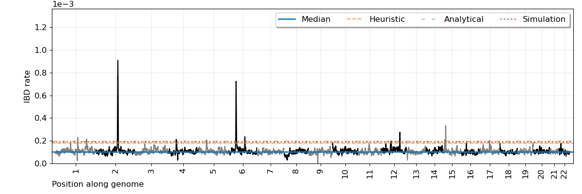
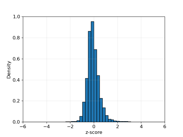
scan.png: the IBD rates along autosomes and the estimated significance thresholdsscan.modified.ibd.tsv: the difference in IBD rates along the autosomes in tabular formatautocovariance.png`: model fit for autocovariances of IBD rateszhistogram.png: an empirical distribution of IBD rates (should look Gaussian)roi.tsv: summary table of the genome-wide significant locifwer.analytical.txt: details about parameters and estimates for multiple testingchromosome-sizes-kept.tsv: numbers and cM sizes of chromosomes analyzedibdsegs/: folder and subfolders with detected IBD segments
The main selection scan figure is:
Description of key columns in the scan.modified.ibd.tsv file:
BPWINDOW: base pair locationCMWINDOW: centiMorgan locationCOUNT: number of overlapping IBD segmentsZ: standardized IBD ratePVALUE: the p value which is valid asymptoticallyUPPER: an IBD count-based thresholdZ_UPPER: a standardized IBD rate-based thresholdGW_LEVEL: genome-wide significance threshold_ANALYTICAL: discrete-spacing analytical approach_SIMULATE: Ornstein-Uhlenbeck simulation-based approach_CONTINUOUS: continuous-spacing analytical approach (very conservative)ADJ_MEAN: mean IBD countADJ_STDDEV: standard deviation of IBD count
Description of columns in the roi.tsv file:
NAME: autogenerated locus nameCHROM: chromosome numberMAXCOUNT: maximum significant IBD count in the locusMINCOUNT: minimum significant IBD count in the locusBPCENTER: base pair where the max IBD count isCMCENTER: centiMorgan where the max IBD count isCMLEFT: centiMorgan where the locus ends on the leftCMRIGHT: centiMorgan where the locus ends on the rightBPLEFTCENTER: same asCMLEFTexcept plus a buffer if locus is too small for hard sweep modelingMODEL: autogenerated as additive genic selection for hard sweep modelingINTERVALCOVERAGE: autogenerated as 95 percent confidence intervals for hard sweep modeling
Note
The multiple-testing corrections are valid asymptotically (Temple and Thompson, 2024+). You can look at the IBD rate histogram to visually assess such (example below). Be wary of IBD rates being zero truncated in small samples.
Note
You can look at the autocovariance.png files to see if the IBD rate decay fits the Ornstein-Uhlenbeck well.

Note
There is a multiprocessing version using Snakefile-scan-mp.smk, which may only be useful in enormous human biobanks.
Modeling hard sweeps
The worfklow/model-selection estimates frequencies, locations, and selection coefficients of loci detected in the Selection scan. This workflow must be run after the selection scan. You should use the Snakefile-roi.smk file as input to the -s option.
The recipe YAML file to modify is sweep.yaml. There is a hierarchy of change versus fixed parameters, where change you should modify for your dataset and fixed you should reach out for advice.
The main command is
nohup snakemake -s Snakefile-roi.smk [...] --cluster "sbatch [...]" --jobs XX --configfile sweep.yaml
The parameters are:
Many parameters under
filesdetermine where your data is and where you want outputs to be.regions_of_interest: these are the loci to analyse. The default are those GW significant in the scan. You can delete some, or rename the GW significant “hits”.chromosome_prefix: this is the namechror blank that you see when you runbcftools query -f "%CHROM\n" chr.vcf.gz | head.ploidy: if your ploidy is not 1 or 2, see Ploidy extensionNe: an estimate of recent effective population sizes (IBDNe text file format)
You can change the genic selection model in roi.tsv to “a” for additive, “m” for multiplicative, “d” for dominance, and “r” for recessive. You can also change alpha, which determines the (1-alpha) percent confidence intervals.
The script scripts/run-ibdne.sh runs IBDNe, which is good for populations with exponential growth. You may want to consider another Ne estimator as well.
sbatch [...] run-ibdne.sh [ibdne-jar] [memory-in-Gb] [main-folder-of-study] [path-to-subfolder-with-ibd-data] [chromosome_low] [chromosome_high] [output_file] [random_seed]
The outputs are:
summary.hap.norm.tsv: sweep model estimates for best haplotype-based analysis and Gaussian confidence intervals for selection coefficientsummary.snp.norm.tsv: sweep model estimates for best SNP-based analysis and Gaussian confidence intervals for selection coefficienthit*/second.ranks.tsv.gz: alleles with putative evidence for selection (or strong correlation with a selected allele)hit*/outlier*.txt: files with sample haplotype IDs in clusters on excess IBD sharing
Description of columns in summary.*.*.tsv files:
MAXCOUNT: maximum IBD count from the selection scanINTERVALCOVERAGE: The (1 - alpha) percent coverage of confidence interval (e.g. 95 percent)LOCHAT: Base pair estimate of a putative sweeping alleleCOUNTIBD: IBD count at the base pair estimatePHAT: Sweeping allele frequency estimateSHAT: Selection coefficient estimateCONF_INT_LOW: If s in (A,B) is the confidence interval, this value is ACONF_INT_UPP: If s in (A,B) is the confidence interval, this value is BMODEL: a for additive, m for multiplicative, d for dominance, r for recessiveGINI_IMPURITY: Gini impurity of the excess IBD sharing groupNUM_OUTLIER_GROUPS: number of disconnected clusters in excess IBD sharing groupPROP_IN_OUTLIER_GROUP: fraction of sample haplotypes in excess IBD sharing group
Note
The Gaussian bootstrap intervals are valid asymptotically (Temple and Thompson, 2024+). You can uncomment lines in rule all of the Snakefile-roi.smk to get percentile-based bootstrap intervals.
All of the IBD clusters are in the files communities.csv. Each cluster is a comma-separated cluster with sample haplotype IDs. The _1 and _2 suffixes correspond to the haplotypes of a diploid individual.
Note
If NUM_OUTLIER_GROUPS is more than a few, GINI_IMPURITY exceeds 0.6, or PROP_IN_OUTLIER_GROUP is less than 0.10, the significant locus may not be the result of a hard sweep. The outliers.py method has been modified to call the largest cluster the excess IBD group if no cluster satisfies the heuristic. This behavior could explain a small PROP_IN_OUTLIER_GROUP value. This behavior may also identify haplotypes from one sweep where there may be multiple sweeps.
Description of columns in second.ranks.tsv.gz files:
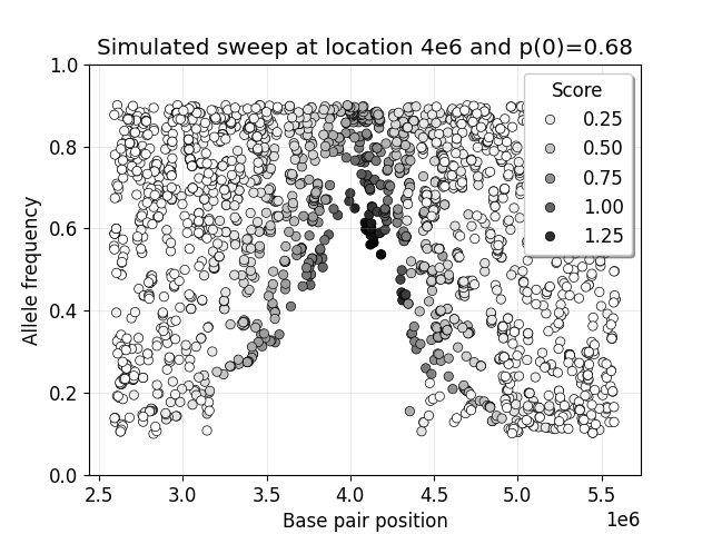
POS: marker locationAAF: allele frequency in entire sampleAAF1: allele frequency in excess IBD sharing groupAAF0: allele frequency in the rest of the sampleZDELTA: this value isAAF1minusAAF0divided by square rootAAFtimes one minusAAF
You can use the values in this table and the notebook scripts/model/telltale-v2.ipynb to make plots like below. The decay of intermediate frequencies is good evidence of a sweep.
Case-control scan
The worfklow/scan-case-control implements the difference in IBD rates scan with two multiple-testing corrections. You should use the Snakefile-case.smk file as input to the -s option.
You must run this workflow after the selection scan workflow (where the IBD segments are detected). You should scrutinize the results to see if strong selection confounds your case-control study.
The recipe YAML file to modify is case.yaml. The parameters are nearly all the same as in Selection scan. The case parameter is a two-column text file with sample IDs and binary phenotypes.
The main command is
nohup snakemake -s Snakefile-case.smk [...] --cluster "sbatch [...]" --jobs XX --configfile case.yaml.
The outputs have the same nomenclature as in the selection scan workflow, but .case. and .control. is inserted in file names:
scan.case.control.png: the standardized difference in IBD rates along autosomes and the estimated significance thresholdsscan.case.ibd.tsv: the difference in IBD rates along the autosomes in tabular formatroi.case.tsv: summary table of the genome-wide significant locifwer.analytical.case.txt: details about parameters and estimates for multiple testing
Note
The multiple-testing corrections are valid asymptotically (Temple and Thompson, 2024+). You can look at the IBD rate histogram to visually assess such. Be wary of IBD rates being zero truncated in small samples.
Note
There is a multiprocessing version using Snakefile-case-mp.smk, which may only be useful in enormous human biobanks.
Note
There is a version with a randomization test using Snakefile-case-randomized.smk and case.randomized.yaml as the template YAML containing a parameter num_randomized. This could be computationally intensive in enormous human biobanks.
Note
The randomization test is not a valid way to get the genome-wide significance threshold if there are true positive signals or loci under strong selection. You can identify confounding in the output scan.randomized.ibd.tsv file if there are loci significant in many runs of randomized phenotypes.
You can try to detect clusters of cases or controls with excess IBD sharing GW significant loci using Snakefile-case-roi.smk and the template --configfile case.roi.yaml.
The output to this feature will be a tab-separated file with sample haplotype IDs, their binary phenotype, and indicators if they are in excess IBD sharing groups (matrix.outlier.phenotypes.tsv for each hit). An example of this file is design.sorted.tsv. You could perform regression analyses on these dataframes. Scripts scripts/utilities/fake-phenotypes-*.py can be used for testing and evaluating confounding from strong recent selection.
You can also look at the sample haplotype IDs in the hit*/outlier*.phenotype.tsv files.
Note
I tested that Snakefile-case-roi.smk runs smoothly, but not if it works well at its task in a simulation study.
Phasing and ancestry
This worfklow/phasing-ancestry provides support for automated haplotype phasing (Beagle), local ancestry inference (Flare), and kinship inference (IBDkin).
The main command is
nohup snakemake -s Snakefile-*.smk [...] --cluster "sbatch [...]" --jobs XX --configfile phasing-and-lai.yaml
The Snakefiles are:
Snakefile-beagle-flare-gds.smk: your data is stored as GDS files, and you want to phase as well as LAI and IBD inferenceSnakefile-beagle-flare-vcf.smk: your data is stored as VCF files, and you want to phase as well as LAI and IBD inferenceSnakefile-flare-only-gds.smk: your data is already phased in GDS files, and you want to perform LAI and IBD inferenceSnakefile-flare-only-vcf.smk: your data is already phased in VCF files, and you want to perform LAI and IBD inference
The YAML example file is phasing-and-lai.yaml. Most of the parameters are written exactly as the parameters in Beagle, Flare, or hap-ibd. Other parameters define file locations. The remaining parameters are:
rename-chrs-map-adx,rename-chrs-map-ref: harmonizes 9 vs chr9 in VCF CHROM column with genetic map. Files are inrename-chrs/. Thenum-chrnum.txtmeans 9 is in the VCF column, but chr9 is in the genetic map column.ref-panel-map: tab-separated, headerless file with reference sample ID (column 1) and reference panel label (column 2)keep-samples: the sample IDs to phase, LAI, and IBD infer, which may be a subset of a larger consortium datasetbcftools-parameters:c-min-mac: minimum minor allele count, where 1 and 2 are incredibly difficult to phase
Note
We strongly recommend against setting flare-parameter:probs equal to true, which may create enormous file sizes and require a lot of RAM.
Note
The output files are in gtdata/, lai/, and ibdsegs/. Rephasing is unphasing the reference panel and phasing them again with all the admixed samples; reference phasing is using the existing phase of the reference panel. Rephasing takes longer and creates more disk memory. You can uncomment or comment these output files in the rule all of the Snakefile.
Note
You can use run-ibdkin.sh (with IBDkin), high-kinship.py, and keep-one-family-member.py in scripts/pre-processing/ to filter out close relatives, say kinship >= 0.125. These scripts are not documented, so I recommend copy and paste into an LLM and ask it what these do.
Publication-ready Figures
Here, I provide some examples terminal commands to make publication-ready figures. The pipelines make some initial plots, but you may want to modify labels and colors. Many of the terminal options are the options in the Python matplotlib library.
This script makes figures for selection scans.
python scripts/plotting/plot-scan-pipeline.py \
   --input_file scan.modified.ibd.tsv \
   --output_prefix scan \
   --sample_size 13778 \
   --ploidy 2 \
   --heuristic_cutoff 4. \
   --num_sims 500 \
   --chr_low 1 \
   --chr_high 22 \
   --statistic COUNT \
   --title "TOPMed European ancestry" \
   --xlabel "Base pair along autosomes" \
   --ylabel "IBD rate" \
   --rotation 90 \
   --yupp 2e-4 \
   --alpha 0.25 \
   --fontsize 14 \
   --width 12 \
   --height 4
Note
If --num_sims is 0, no simulation-based threshold will be plotted. Any value of --num_sims greater than 0 will plot the simulation-based threshold in scan.modified.ibd.tsv.
Note
You could use this script, or scripts/plotting/plot-scan.py as a general use plotter. However, you would need be careful with the --sample_size and --statistic parameter. For instance, you could augment the scan.case.ibd.tsv file with a simulation-based threshold.
This script makes figures for IBD mapping / case-control scans.
python scripts/plotting/plot-scan-case-pipeline.py \
   --input_file scan.case.ibd.tsv \
   --output_prefix scan.case \
   --chr_low 1 \
   --chr_high 22 \
   --statistic ZDIFFZ \
   --title "ADSP European ancestry" \
   --xlabel "Base pair along autosomes" \
   --ylabel "Standardized IBD rate difference" \
   --rotation 90 \
   --yupp 8. \
   --alpha 0.25 \
   --fontsize 14 \
   --width 12 \
   --height 4
This script plots the empirical distribution of IBD rates of IBD rate differences.
python scripts/plotting/plot-histogram.py \
   --input_file scan.modified.ibd.tsv \
   --output_file histogram.png \
   --chr_low 1 \
   --chr_high 22 \
   --chrom CHROM \
   --statistic COUNT \
   --outlier_cutoff 1000
Note
We reuse this plotter for the case-control scan, changing --statistic to ZDIFFZ.
Note
The --outlier_cutoff option, in normally-distributed quantiles, is used to remove outliers before standardizing.
This script plots autocovariance by genetic distance.
python scripts/plotting/plot-autocovariance.py \
   --input_autocov_file fwer.autocovariance.tsv \
   --input_analytical_file fwer.analytical.tsv \
   --output_prefix autocovariance \
   --theta_type estimated-theta: \
   --title "TOPMed European ancestry" \
   --xlabel "Genetic distance (cM)" \
   --ylabel "Autocovariance" \
   --yupp 1.5 \
   --color tab:blue \
   --width 6.4 \
   --height 4.8
Note
If your --input_analytical_file is fwer.analytical.case.tsv, you may use estimated-theta0: or estimated-theta1: to plot results for case and control sample sets. You must also modify the input_autocov_file parameter.
Note
We reuse this plotter for the case-control scan, changing the --input_autocov_file and --input_analytical_file.
This script makes figures for sweep modeling.
python scripts/plotting/plot-sweep.py \
   --output_file sweep.LCT.png \
   --s 0.03 \
   --su 0.04 \
   --z \
   --p 0.70 \
   --Ne ibdne.ne \
   --standing_variation -0.01 \
   --genetic_model a \
   --ploidy 2 \
   --nboot 1000 \
   --upper_quantile 0.99 \
   --lower_quantile 0.01 \
   --xaxis_length 150 \
   --line_color tab:blue \
   --font_size 14 \
   --alpha 0.25 \
   --title "LCT gene"
The parameters are:
--sestimate of selection coefficient
--suthe upper bound of selection coefficient confidence interval
--zthis corresponds to to the quantile of a N(0,1), e.g. 1.96 for 95 percent confidence intervals
--pestimate of sweeping allele frequency
--Nefile with estimates of population effective sizes
--standing_variationpositive selection stops once this allele frequency is reached
--genetic_modela for additive, m for multiplicative, d for dominance, r for recessive
--nbootnumber of Wright-Fisher simulations with selection
--upper_quantileand--lower_quantileconcern the sweep frequency intervals
--xaxis_lengthis the number of generations
Note
You should get these parameters from summary.hap.norm.tsv or summary.snp.norm.tsv files. The plotter assumes normally-distributed confidence interval, which is only reasonable when Temple and Thompson conditions hold.